The titanic problem is easily one of the most popular competitions on Kaggle and a great project to get your hands dirty with as an upcoming data scientist. This breakdown of the project includes some tips and tricks to help get over 70% accuracy. Improving on that would be left to you.
The objective is an accurate prediction of survivors among the passengers of the Titanic. In this notebook, 82.26% is the best score on the training set using Logistic regression, while 0.77 is the public score.
Below is an overview of the steps taken
- Data exploration
- Data cleaning
- Feature engineering
- Data preprocessing
- Model development and comparison
- Results
- Submission
- Data exploration
Let’s read our training data and have a look at the first ten rows. The aim here is to have a proper idea of the type of data contained in each column.
import numpy as np # linear algebra
import pandas as pd # data processing, CSV file I/O (e.g. pd.read_csv)df=pd.read_csv('/kaggle/input/titanic/train.csv')
df

Now let’s check for null/missing values.
l=df.isnull().sum()
print(l , df.shape)
We can now see the number of missing values in the ‘Age’ column, ‘Cabin’ and ‘Embarked’ column; later, we would do some imputations to handle them.
The cell below contains code to check the degree of correlation between the columns; take note that each column is expected to be perfectly correlated with itself. The columns with the most correlation are the ‘SipSp’ (sibling to parent ratio) column and ‘Parch’ (parent to children ratio) columns.
import seaborn as sns
sns.heatmap(df.corr())

We would need to have a good understanding of our data. Thus, we would be exploring the survival rates (the dependent variable) for each column (independent variables).
Let’s first have a look at the overall survival rate.
sns.countplot(data=df, x='Survived')
From the plot above, it is clear that more people died than survived; over 500 passengers died while less than 400 survived. Let us look at how the independent variables (sex, age, embarked, fare, Pclass, etc) are related to the survival rate. We would be starting with sex.
The plots below show the survival rate with respect to sex. The plot on the left shows the total number of males and females that boarded the ship while the one on the right shows the number of males and females that survived or not. Less than 110 (20 percent) of the males on the ship survived while over 200 (70 percent) of the females survived. Hence a female has a higher chance of survival (4 times more) than a male.
from matplotlib import pyplot as plt
fig, axes = plt.subplots(1,2, figsize=(20,5))
sns.countplot(ax=axes[0], data=df,x='Sex')
sns.countplot(ax=axes[1],data=df,x='Sex',hue='Survived')
we can go ahead to check the survival rate with respect to the point of embarkment
sns.set_palette('Paired')
fig, axes = plt.subplots(1,2, figsize=(20,5))
sns.countplot(ax=axes[0], data=df,x='Embarked')
sns.barplot(ax=axes[1],data=df, x= 'Embarked', y='Survived')
The plot on the left shows the total number of passengers that embarked from different points, with ‘nan’ representing passengers whose point of embarkment is not on record. The plot on the right represents the percentage of passengers that survived from each point of embarkment. From the barplot, it is evident that passengers that embarked at ‘C’ had a higher chance of survival, 55% of them survived, meanwhile fewer than 40% of the passengers that embarked at ‘S’ and ‘C’ survived with ‘S’ having the lowest survival rate (note that very few passengers had their point of embarkment not recorded, and they all survived).
Below is a look at the survival rate of men and women with respect to where they embarked.
sns.set_palette('Paired')
fig, axes = plt.subplots(1,2, figsize=(20,5))
sns.countplot(ax=axes[0], data=df,x='Embarked', hue='Survived')
sns.barplot(ax=axes[1],data=df, x= 'Embarked', y='Survived', hue='Sex')
The plot above shows that more females that embarked from each category survived.
Let’s go ahead and check survival rate with respectc to a passengers class (Pclass).
fig, axes = plt.subplots(1,2, figsize=(20,5))
sns.countplot(ax=axes[0], data=df,x='Pclass')
sns.barplot(ax=axes[1], data=df,x='Sex',y='Survived', hue="Pclass")
From the plots, it is evident that more passengers were in the passenger class ‘3’ while the least amount of passengers were in class ‘2’. Conversely, male and female passengers in passenger class ‘3’ had the lowest chance of survival while those in class ‘1’ had the highest possibility of survival.
Up next we would be checking the survival rate by age.
sns.histplot(data=df,x='Age')
Knowing we have over 800 passengers, below is the age distribution of our passengers. The majority of the passengers fall within the ages of 15 to 40 years. If we plot the relationship between age and survival, we would have a cluttered graph due to a wide range of different values for the fares. Hence we would be splitting the fares into fare groups in a new column. Now we create a column where we group the ages in groups of 10 and sort them for easy plotting, and a clear graph showing the survival rate concerning age and sex.
Age_group=[]
for c in df.Age:
    if c<11:
        Age_group.append("0-10")
    elif 10<c<21:
        Age_group.append("11-20")
    elif 20<c<31:
        Age_group.append("21-30")
    elif 30<c<41:
        Age_group.append("31-40")
    elif 40<c<51:
        Age_group.append("41-50")
    elif 50<c<61:
        Age_group.append("51-60")
    elif 60<c<71:
        Age_group.append("61-70")
    else:
        Age_group.append("71-80")

df['age_group']=Age_groupfig, axes = plt.subplots(1,2, figsize=(20,5))
sns.set_palette('Paired')
df1=df.sort_values('Age', ascending=True)
sns.countplot(ax=axes[0], data=df1,x='age_group', hue="Survived")
sns.barplot(ax=axes[1], x='age_group', hue='Sex', data=df1, y='Survived')

From the graph on the left, we can see that most of the survivors were within the age group of 21–30 years, while those within 61–70 survived least. From the graph on the right, males within the age group of 0–10 years had almost the same chance of survival as the females in the same age group, and that is the age group for males with the highest possibility of survival. The graph below gives us a clearer view of the age group with the highest chance of survival within males and females.
sns.barplot(data=df, x='Sex',hue='age_group', y='Survived')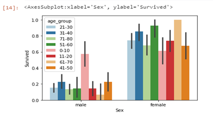
The graph below shows the rate of survival for SibSp (number of siblings/parents), passengers with 0 and 1 ‘SibSP’ have the highest chance of survival; whereas, those with 6 and 8 have the lowest chance of survival (0 possibilities of survival).
fig, axes = plt.subplots(1,2, figsize=(20,5))sns.countplot(ax=axes[0], data=df,x='SibSp')sns.countplot(data=df, x='SibSp', hue='Survived')

looking at the survival rate for ‘Parch’ (number of children/parents) we can see that most of the passengers had 0 ‘Parch’ with 6 being the least. However Passengers with ‘Parch’ of 2 had a 50% chance of survival, which is the highest chance of survival with regards to ‘Parch’.
fig, axes = plt.subplots(1,2, figsize=(20,5))
sns.countplot(ax=axes[0], data=df,x='Parch')
sns.countplot(data=df, x='Parch', hue='Survived')
If we plot the relationship between fares and survival, we would have a cluttered graph due to a wide range of different values for the fares. Hence we would be splitting the fares into fare groups in a new column.
fare_group=[]
for c in df.Fare:
    if c<11:
        fare_group.append("0-10")
    elif 10<c<21:
        fare_group.append("11-20")
    elif 20<c<31:
        fare_group.append("21-30")
    elif 30<c<41:
        fare_group.append("31-40")
    elif 40<c<51:
        fare_group.append("41-50")
    elif 50<c<101:
        fare_group.append("50-100")
    elif 100<c<201:
        fare_group.append("101-200")
    elif 200<c<301:
        fare_group.append("201-300")
    elif 300<c<401:
        fare_group.append("301-400")
    elif 400<c<501:
        fare_group.append("401-500")
    else:
        fare_group.append("501-550")

df['Fare_group']=fare_group
df['Fare_group'].value_counts()#output below0-10       364
11-20      160
21-30      142
50-100     106
31-40       50
101-200     33
201-300     17
41-50       16
501-550      3
The output cell above shows the count for each fare group; we can go ahead and sort the fare_group column then plot graphs using the fare_group columns
df2=df.sort_values('Fare', ascending=True)
fig, axes = plt.subplots(1,2, figsize=(20,5))
sns.barplot(ax=axes[1], x='Fare_group', hue='Sex', data=df2, y='Survived')
sns.countplot(ax=axes[0],data=df2, x='Fare_group', hue='Survived')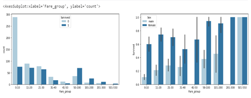
From the graphs above, more passengers paid between 0–10, and females had a higher survival rate in each fare group, excluding those that paid within 501–550 where everyone survived.
DATA CLEANING
Let’s have a look at where we have null values.
df.drop(['age_group','Fare_group'], axis=1,inplace =True)
d=df.isnull().sum()
d#output
PassengerId      0
Survived         0
Pclass           0
Name             0
Sex              0
Age            177
SibSp            0
Parch            0
Ticket           0
Fare             0
Cabin          687
Embarked         2
We have a large number of null values, so dropping them would not be a smart move as that would mean losing over half of our data. Hence we would be doing some imputation. However, let’s first have a good look at our test set.
test_data=pd.read_csv('/kaggle/input/titanic/test.csv')
test_data.head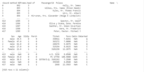
To make our job easy when cleaning, preprocessing, and carrying out imputations, we would be joining our test and train sets together to carry out the earlier mentioned steps once without the need for repeating any operation for both the training and test set.
all_data=pd.concat([df,test_data], ignore_index=True)  # we are setting the ignore_index to true so our combined data set would be indexed continously (indexed from 0_1309)
all_data.head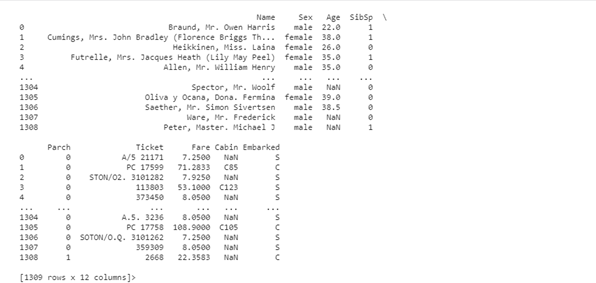
Now that we have combined our data set, let’s look at a summary of each column so we identify columns with missing values.
all_data.info()#output
<class 'pandas.core.frame.DataFrame'>
RangeIndex: 1309 entries, 0 to 1308
Data columns (total 12 columns):
 #   Column       Non-Null Count  Dtype
---  ------       --------------  -----
 0   PassengerId  1309 non-null   int64
 1   Survived     891 non-null    float64
 2   Pclass       1309 non-null   int64
 3   Name         1309 non-null   object
 4   Sex          1309 non-null   object
 5   Age          1046 non-null   float64
 6   SibSp        1309 non-null   int64
 7   Parch        1309 non-null   int64
 8   Ticket       1309 non-null   object
 9   Fare         1308 non-null   float64
 10  Cabin        295 non-null    object
 11  Embarked     1307 non-null   object
dtypes: float64(3), int64(4), object(5)
memory usage: 122.8+ KB
The ‘Embarked’ column is missing two columns (has 1307 out of 1309 values), while the ‘Cabin’ columns are missing over 1000 values, while the ‘Age’ column is missing just over 200 values. Let us start our imputations on the Embarked column.
all_data.Embarked.unique()#output
array(['S', 'C', 'Q', nan], dtype=object)
The cell above shows us all unique values from the Embarked column, we can see that the column contains ‘nan’ values. Let’s write a code to replace the nan values with those having maximum occurrence. The cell below checks the count of all values in the column.
all_data.value_counts()
‘S’ occurs more than any other value, therefore we would be replacing the ‘nan’ values with ‘S’. We first have to get the location of the ‘nan’ values, that is what’s done in the cell below.
for i,j in enumerate(all_data.Embarked):  # gettin a value pair of each value (i) and its index location (j)
    if type(j)!=str:
        print(i,j)#ouput
61 nan
829 nan
Now that we have the index of the ‘nan’ values, we can input the value with the highest frequency, which is ‘S’ and we check if our imputation was a success
all_data.Embarked[61]='S'
all_data.Embarked[829]='S'
all_data.Embarked.value_counts()#output
S    916
C    270
Q    123
Name: Embarked, dtype: int64
There is only a single missing value in the ‘Fare’ column. The cell below checks all the rows in the ‘Fare’ column for the missing value and replaces it with the mean of all values in the column.
for i,j in enumerate(all_data.Fare):  # gettin a value pair of each value (i) and its index location (j)
    if np.isnan(j):
         all_data.Fare[i]=test_data.Fare.mean()
print(all_data.Fare[i])#output
22.3583
To fill the values in the ‘Age’ column, we would be taking a different approach, grouping the passengers by sex, Pclass, and Embarked before getting their mean age for each group. This should give us a better result than just generalizing the mean age for all the passengers. We would be using the group_by method to actualize this.
df1=all_data.groupby(['Sex','Pclass','Embarked']).mean()
df1

The next thing is the replace the null (nan) values with the mean age for their respective groups. The cell below contains a loop that scans through all rows in the ‘Age’ column, checking the group they belong to and imputing the mean age for that group. ( ias the passager a male, what is his Pclass and finally where did he embark from, before imputing the mean age for passengers from that group).
for j,i in enumerate(all_data.Age): # gettin a value pair of each value (i) and its index location (j)
    if np.isnan(i):   # checking if the value is a null (nan) value
        if all_data.Sex[j]=='female':   #check the sex using the index (j) locaion
            if all_data.Pclass[j] == 1:  # check the Pclass using the index (j) locaion
                if all_data.Embarked[j]=='C':  # check where the passenger embarked from using the index (j) locaion
                    all_data.Age[j]=38  # impute mean age for that group using the index (j) locaion
                if all_data.Embarked[j]=='Q':
                    all_data.Age[j]=35
                if all_data.Embarked[j]=='S':
                    all_data.Age[j]=35
            if all_data.Pclass[j] == 2:
                if all_data.Embarked[j]=='C':
                    all_data.Age[j]=23
                if all_data.Embarked[j]=='Q':
                    all_data.Age[j]=30
                if all_data.Embarked[j]=='S':
                    all_data.Age[j]=28
            if all_data.Pclass[j] == 3:
                if all_data.Embarked[j]=='C':
                    all_data.Age[j]=15
                if all_data.Embarked[j]=='Q':
                    all_data.Age[j]=22
                if all_data.Embarked[j]=='S':
                    all_data.Age[j]=22
        if all_data.Sex[j]=='male':
            if all_data.Pclass[j] == 1:
                if all_data.Embarked[j]=='C':
                    all_data.Age[j]=39
                if all_data.Embarked[j]=='Q':
                    all_data.Age[j]=44
                if all_data.Embarked[j]=='S':
                    all_data.Age[j]=42
            if all_data.Pclass[j] == 2:
                if all_data.Embarked[j]=='C':
                    all_data.Age[j]=29
                if all_data.Embarked[j]=='Q':
                    all_data.Age[j]=59
                if all_data.Embarked[j]=='S':
                    all_data.Age[j]=29
            if all_data.Pclass[j] == 3:
                if all_data.Embarked[j]=='C':
                    all_data.Age[j]=24.25
                if all_data.Embarked[j]=='Q':
                    all_data.Age[j]=25
                if all_data.Embarked[j]=='S':
                    all_data.Age[j]=25
Lets check if our imputation for the age column was sucessfull
all_data.info()#output
<class 'pandas.core.frame.DataFrame'>
RangeIndex: 1309 entries, 0 to 1308
Data columns (total 12 columns):
 #   Column       Non-Null Count  Dtype
---  ------       --------------  -----
 0   PassengerId  1309 non-null   int64
 1   Survived     891 non-null    float64
 2   Pclass       1309 non-null   int64
 3   Name         1309 non-null   object
 4   Sex          1309 non-null   object
 5   Age          1309 non-null   float64
 6   SibSp        1309 non-null   int64
 7   Parch        1309 non-null   int64
 8   Ticket       1309 non-null   object
 9   Fare         1309 non-null   float64
 10  Cabin        295 non-null    object
 11  Embarked     1309 non-null   object
dtypes: float64(3), int64(4), object(5)
From the above we have 1309 non null values, which is the total number of values in the column.
FEATURE ENGINEERING
In this section, we would generate new features (columns) from the existing features. THE AIM OF THIS IS TO DEVELOP HELPFUL FEATURES WHICH CAN IMPROVE OUR PREDICTIONS.
Starting with the ‘Cabin’ column where we have a lot of missing values, the cabin numbers are arranged in a string_integr pair, so we can take the first letter of each cabin number and use that as a cabin class/group, while the ‘nan’ values are taken as a separate group thereby creating a new feature/column with no missing values.
all_data['cabin_adv'] = all_data.Cabin.apply(lambda x: str(x)[0]) # we use the 'str' method to strip the cabin number and take only the first character (the same applies for 'nan' values).
all_data.info()#output
<class 'pandas.core.frame.DataFrame'>
RangeIndex: 1309 entries, 0 to 1308
Data columns (total 13 columns):
 #   Column       Non-Null Count  Dtype
---  ------       --------------  -----
 0   PassengerId  1309 non-null   int64
 1   Survived     891 non-null    float64
 2   Pclass       1309 non-null   int64
 3   Name         1309 non-null   object
 4   Sex          1309 non-null   object
 5   Age          1309 non-null   float64
 6   SibSp        1309 non-null   int64
 7   Parch        1309 non-null   int64
 8   Ticket       1309 non-null   object
 9   Fare         1309 non-null   float64
 10  Cabin        295 non-null    object
 11  Embarked     1309 non-null   object
 12  cabin_adv    1309 non-null   object
dtypes: float64(3), int64(4), object(6)
memory usage: 133.1+ KB
We can also extract the title of each passenger from their names and create a separate column for that. Let us have a look at how the names are arranged first.
all_data.Name.head#output
<bound method NDFrame.head of 0                                 Braund, Mr. Owen Harris
1       Cumings, Mrs. John Bradley (Florence Briggs Th...
2                                  Heikkinen, Miss. Laina
3            Futrelle, Mrs. Jacques Heath (Lily May Peel)
4                                Allen, Mr. William Henry
                              ...
1304                                   Spector, Mr. Woolf
1305                         Oliva y Ocana, Dona. Fermina
1306                         Saether, Mr. Simon Sivertsen
1307                                  Ware, Mr. Frederick
1308                             Peter, Master. Michael J
Name: Name, Length: 1309, dtype: object>
The names are in the format of Name/Tittle/Other Names. Hence, we split the names at the first ‘comma’ and pick the title, then we split the title of the ‘full stop’ at its end and take the title alone as in the first line of the cell below.
ll_data['tittle'] = all_data.Name.apply(lambda x: x.split(',')[1].split('.')[0].strip())
all_data.info()#output
RangeIndex: 1309 entries, 0 to 1308
Data columns (total 14 columns):
 #   Column       Non-Null Count  Dtype
---  ------       --------------  -----
 0   PassengerId  1309 non-null   int64
 1   Survived     891 non-null    float64
 2   Pclass       1309 non-null   int64
 3   Name         1309 non-null   object
 4   Sex          1309 non-null   object
 5   Age          1309 non-null   float64
 6   SibSp        1309 non-null   int64
 7   Parch        1309 non-null   int64
 8   Ticket       1309 non-null   object
 9   Fare         1309 non-null   float64
 10  Cabin        295 non-null    object
 11  Embarked     1309 non-null   object
 12  cabin_adv    1309 non-null   object
 13  tittle       1309 non-null   object
dtypes: float64(3), int64(4), object(7)
Checking for null values in our dataset we can see that there are no null values except in the ‘Cabin’ column, and this is not a problem as we would be using our ‘cabin_adv’ column instead. We can also see the new columns we created (title, cabin_adv).
We would be doing something similar to our ticket column as done to our cabin column. We would take the first letter of our string_integer pair and use it to create a new feature/column as our ticket class. Let us first have a look at how the tickets are arranged.
all_data.Ticket.head(20)#output
0            A/5 21171
1             PC 17599
2     STON/O2. 3101282
3               113803
4               373450
5               330877
6                17463
7               349909
8               347742
9               237736
10             PP 9549
11              113783
12           A/5. 2151
13              347082
14              350406
15              248706
16              382652
17              244373
18              345763
19                2649
Name: Ticket, dtype: object
Now lets create our new column/feature
all_data['ticket_typ']= all_data.Ticket.apply(lambda x: x.split('/')[0]) #split the ticket at '/' and take the first value
all_data['ticket_typ']= all_data.Ticket.apply(lambda x: x.split(' ')[0]) #split the ticket(the output above) at ' ' (space) and take the first value

for i,t in enumerate(all_data.ticket_typ):  # this loop checks the length of the tickets and picks only the first character if the length  id more than 1. if the first character is a number it replaces it with 'x' otherwise it keeps it if is an alphabet
    if len(t)>1:
        all_data.ticket_typ[i]= t[0]
        if t[0].isdigit():
            all_data.ticket_typ[i]='x'
all_data.ticket_typ.value_counts()#output
x    957
S     98
P     98
C     77
A     42
W     19
F     13
L      5
Name: ticket_typ, dtype: int64
Now let’s split our data set (all_data) into training and test set so we can look at the distributions of our columns with imputations done in our new columns.
train=all_data.iloc[0:891,:] # our training set had 891 rows, it occupies the forst 891 rows of our combined data set
train

test=all_data.iloc[891:,:] # our test set had 418 rows, it occupies the last 418 rows of our combined data set
test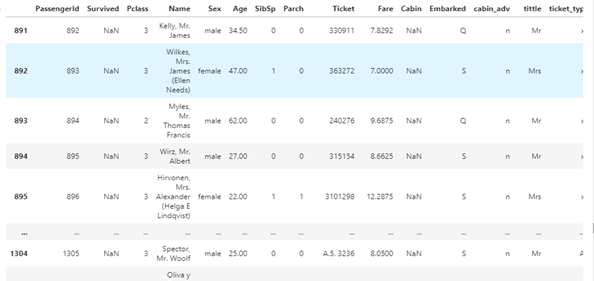
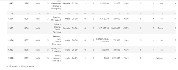
Checking the cabin_adv (cabin group/class), it is evident that the ’n’ class/group had more passengers. However, the ‘E’, ‘D’, and ‘F’ classes/groups had the best survival rates even though they had far fewer passengers.
fig, axes = plt.subplots(1,2, figsize=(20,5))
sns.barplot(ax=axes[1], x='cabin_adv', data=train, y='Survived')
sns.countplot(ax=axes[0],data=train, x='cabin_adv', hue='Survived')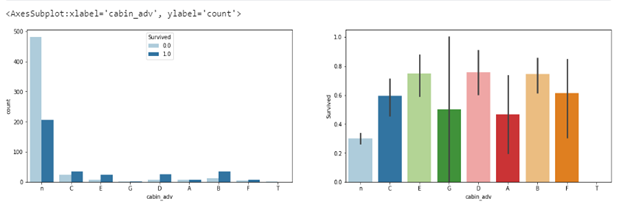
Below is a table showing survival rates by tittle, nan represents 0
pd.pivot_table(train,index='Survived',columns='tittle', values = 'Ticket', aggfunc='count')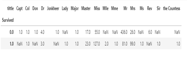
Below is a table showing survival rated by ticket type. Passengers with “P’ tickets had the highest survival rates.
pd.pivot_table(train, index='Survived', columns='ticket_typ', values='Ticket', aggfunc='count')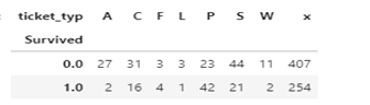
MODEL PREPROCESSING
We would revert to using our combined data set (all_data) for preprocessing, ‘features’ is the list of columns we would be using to train our model. Notice we have dropped the name, passenger_id, tittle, ticket, and cabin column but are using tittle, ticket_typ, cabin_adv instead. This is because the dropped columns are of no use to our model since they are specific to each passenger and we have extracted useful information from them.
features=[ 'Pclass','Sex','Age', 'SibSp',
       'Parch', 'Embarked','Fare', 'cabin_adv', 'tittle','ticket_typ',] # notice this does not contain our Survived column because we are going to save them seperatlyall_data_features=all_data[features]
Now lets get dummy variables for our categorical columns (columns with objects/strings and not numerical values)
all_data_dummies=pd.get_dummies(all_data_features)In the cell below we would be extracting our training set from our combined data set just as done earlier, but saving them as X (independent variables) and y(dependent variables)
X=all_data_dummies.iloc[0:891, : ] # this is being extracted from our combined dataset with dummie variables
y=all_data.Survived.iloc[0:891]# this is being extracted from our combined dataset beefore dropping some columns. it's basically our survived column
let’s have a look at y which is the survived column.
y#OUTPUT
0      0.0
1      1.0
2      1.0
3      1.0
4      0.0
      ...
886    0.0
887    1.0
888    0.0
889    1.0
890    0.0
Name: Survived, Length: 891, dtype: float64
MODEL DEVELOPMENT
Time to import neccessary libraries
from sklearn.model_selection import train_test_split
from sklearn.model_selection import cross_val_score
from sklearn.linear_model import LogisticRegression
Using logistic regression
lr = LogisticRegression(max_iter = 2000)
cv = cross_val_score(lr,X,y,cv=5)
print(cv)
print(cv.mean())#output
[0.82681564 0.8258427  0.79775281 0.80898876 0.85393258]
0.822666499278137
From the outputs of our Logistic regression model, we got an accuracy of 0.8229 which is quite good. Let’s fit our model, make and submit predictions.
model = LogisticRegression(max_iter = 2000)
model.fit(X,y)
predictions=model.predict(test).astype(int)output = pd.DataFrame({'PassengerId': test_data.PassengerId, 'Survived': predictions})
output.to_csv('my_submission.csv', index=False)
print("Your submission was successfully saved!")#output
Your submission was successfully saved
Following the steps above, you should get a public score of 0.77 when you submit your predictions, now it’s up to you to improve on the model to get better results. You can tweak the model, try a different model and even do some data engineering.
Here is the link to my github repo for this project:
https://github.com/usmanbiu/kaggle-titanic.git
I hope you found this post helpful, do not forget to share, clap and check back for more posts. thanks and good luck.